@algorithm decorator and SeriesF, MutSeriesF data types which help to create
algorithms that use this technique. All this provides an effective and convenient way for series processing.
@algorithm, SeriesF and MutSeriesF
Decorator @algorithm is a syntactic sugar that can be applied to a function
definition which is equivalent to writing a class definition of an algorithm inherited from indie.Algorithm class.
More details about how this kind of syntactic sugar works are here.
SeriesF is a data type that represents series of numeric values like prices of
some instrument. Every element of a SeriesF object stores a value at time of some bar on a chart. SeriesF objects
have an interface which gives access to their values with square brackets operator. For example, series of close prices
of some instrument is self.close (where self is an object with Context interface) and current (the last) close
price can be accessed with expression self.close[0]. The close price at the previous candle is self.close[1] and so
on.
Series objects like self.open, self.high, self.low, self.close and self.volume are built-in and read-only. But
Indie lets you create your own series objects, put some values that your algorithm calculates into them and use them in
the further parts of your indicator code. This is exactly what MutSeriesF type is intended to be used for.
Function MutSeriesF.new wraps any primitive number value and returns
an object of MutSeriesF type with that value written into the [0] (the most recent element). This provides access to
previous values of that value in the future Indie invocations. In other words, MutSeriesF data type is what you need
if you want to persist some value over bars.
NOTE: MutSeriesF is a type alias for MutSeries[float] and SeriesF is a type alias for Series[float]. In future
versions of Indie it is planned to support other types for element of those containers besides float.
SMA, Sum and sliding window technique
Now it is a good time to look at some of the algorithms in action. Let us take some very basic indicator like for example Simple moving average (SMA) and see how it works under the hood. To calculate SMA with length=4 of some price series, we have to divide every element of a corresponding sum (with the same length=4) by its length. That is why, first we have to look in detail how sum algorithm could be implemented. The sum of length=4 can be calculated simply. First, the value ofsum_0 (where 0 is the bar index) is
undefined, because at that point there is only one price is available in the input series. Same with the sum_1 and
sum_2. But the value of sum_3 equals to price_0 + price_1 + price_2 + price_3 which is 5 + 2 + 1 + 2 = 10.
So far so good and the next sum value, sum_4, equals to price_1 + price_2 + price_3 + price_4 which is
2 + 1 + 2 + 4 = 9 correspondingly. Finally, in the same manner we calculate sum_5 as
price_2 + price_3 + price_4 + price_5 which is 1 + 2 + 4 + 6 = 13. And so on, this is illustrated on the diagram:
Calculation of a sum in a straightforward (but time-inefficient) way:
sum_4 = sum_3 - price_0 + price_4,
sum_5 = sum_4 - price_1 + price_5 and so on. This other way of calculation is exactly the mentioned before
sliding window technique. It turns out that with larger lengths the second way is way more efficient in terms of time.
And here is the Indie implementation of it:
from indie.algorithms import Sum, Sma.
Now, after we have a Sum algorithm, it is trivial to write SMA as Sma algorithm too:
@algorithm return SeriesF result (or tuple of SeriesF values).
Finally here is the Main entry point of our indicator that plots it on chart:
Series behavior during history vs runtime
Suppose we have an indicator that counts green bars of an instrument on a chart: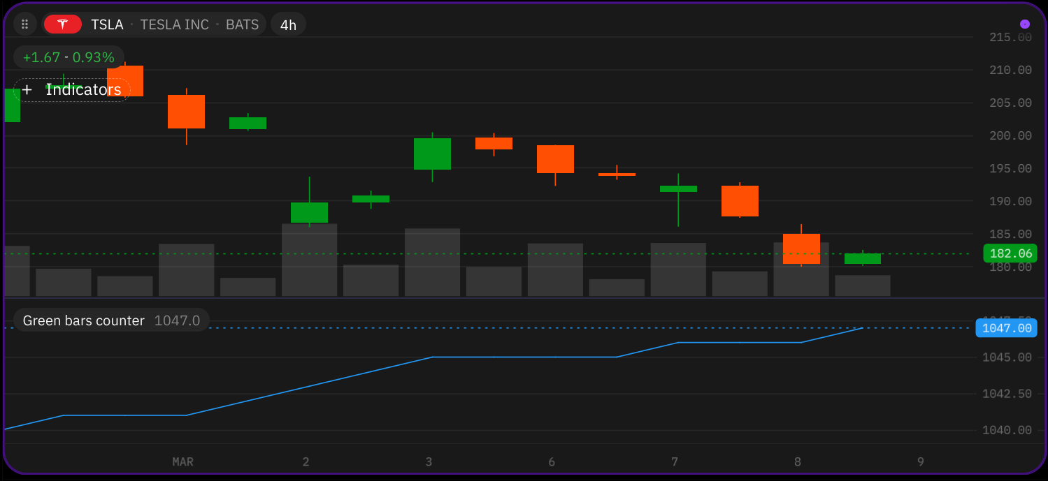
green_count object which accumulates the desired count.
This count is returned from Main which plots a blue line on a chart. On Figure 6.1 we see how blue line rises up by 1
on every green bar and stays flat if bar is red. First let us take a close look at how this Series object behaves during
indicator calculation on a historical bars of some imaginary instrument. Close and open prices of our instrument could
be for example:
open and close will be passed to the indicator for calculation one by one from left to right.
Indicator will calculate, at time t0, like this ‘12 is greater than 9, so we add 1 to green_count’. On the next
calculation, at time t1, it will be ‘7 is not greater than 18, so do nothing. Value of green_count is still 1’. In the
end, green_count series will contain these values:
t6 the real-time begins:
^s. They are important, because values calculated in these moments are
stored in the end in the green_count series, overwriting all values written there before at the time of the same bar.
Bar usually updates multiple times at realtime. Every realtime update of a bar triggers a calculation of indicator.
Right before every such calculation the state of the green_count[0] series element resets to its previous value (i.e.
green_count[1]) — the value it had at the time of previous bar. That is why during the three updates of bar starting
at t6, corresponding element of green_count series was set to 5 at first, then reverted back to 4, then finalized at
value 5.
If nothing is written in the green_count[0] series element and bar finalizes then this value is carried further to
the next series element without change.
MutSeriesF.new() function description
MutSeriesF.new creates MutSeriesF objects which are containers for calculated values in Indie code. The
main feature of MutSeriesF container is ability to store (or ‘remember’) historical values of some variable, those
values could be later accessed with the square brackets operator. At the moment MutSeriesF class supports only
float type as series element.
Please note that MutSeriesF objects give read-write access only to the last value of the series object and read access
to any (well, down to some limit) previous values.
Parameters:
reset— is a value that is written into the most recent element of theMutSeriesFevery timeMutSeriesF.new()function is executed. The effect of this parameter is the same as:
init— is a value that is written into the most recent element of the series object only once after theMutSeriesFobject was created. Or, in other words, it is a value that is written only at the time of the firstMutSeriesF.new()function call.
size— is number of elements thatMutSeriesFobject should persist in memory. The default and minimum possible size is 2, which means that a series of size=2 stores in memory one value at the time of the last candle and another at the time of the previous candle. The size is automatically expanded during the historical calculation of an indicator. For example:
s was expanded from 3 to 6. It is allowed to get access to s[0], s[1], s[2], s[3] and s[4], s[5] elements
after that. It may seem to have not very much sense at first. We set some size, but we are allowed to expand it later.
Well, it is allowed to expand the size only during the calculation of indicator history. The algorithm by some reason
may calculate the lookback offset for some series at runtime, depending on prices for example like this:
self.close series. They could be less than max_size = 100 at first but then during
realtime, they could rise higher. That is why we should always limit the max_offset with min and reserve the s’s
size with size parameter. Otherwise the indicator would fail, since, again, we cannot expand the size at realtime.
NOTE: MutSeriesF objects also have a method request_size(new_size: int) which can be used to expand the size
explicitly.
MutSeriesF.new function has a ‘get or create’ semantics. It means that only one MutSeriesF object is created per one
MutSeriesF.new function call occurrence in the code. All subsequent calls of MutSeriesF.new in exactly the same
position in Indie script simply return MutSeriesF objects created previously. For example:
MutSeriesF objects are created: s1 and s2. The Main function is called multiple times -
per every historical candle and per every realtime update of the last candle — thus multiple times MutSeries.new
functions are called too. But only when self.bar_index == 0 the s1 and s2 objects are created. During all the
subsequent calls, s1 and s2 only receive references to existing MutSeriesF objects. If you want more details about how MutSeriesF.new function works, read this.
TL;DR: How to use classes from indie.algorithms package in my indicator?
Suppose we have found an algorithm (e.g. RSI) in the Indie library and want to use
it in our indicator. These are the steps which should be done in order to achieve this:
- Import the class of the desired algorithm, which in our example let it be the
indie.algorithms.Rsi:
-
Go to the place in the code where you want to call the algorithm. Algorithms can be called either:
- from
Mainentry point or - from secondary context entry point or
- from some other algorithm.
Mainentry point function: - from
new() function from global scope of indicator or from some ‘plain old python
function’.
- Call the algorithm’s
new()syntactic sugar function according to its signature which forRsiisnew(src: indie.SeriesF, length: int) -> indie.SeriesF(here is the link) and write the resulting series of RSI values to some variable, e.g.rsi_result:
- From now you may use the
rsi_resultseries, for example, return it fromMainfor plotting on chart or pass to some other algorithm for further processing. If you want just access the lastfloatRSI value, use square brackets operatorrsi_result[0].
TL;DR: How to use indie.MutSeriesF in my indicator?
Suppose we are working on an indicator where we calculate some math formula on every candle. Let us take something simple like OC2 = (OpenPrice + ClosePrice) / 2 as an example of such a formula. Here is Indie code that calculates and plots OC2:
OC2 variable is float.
It could be very useful to store such a value like OC2 (or, to be more accurate, a series of values because we
calculate new value on each candle) in a Series-like container (which is indie.MutSeriesF). This gives following
benefits:
- it will be possible to access historical values of
OC2(values which were calculated previously on historical candles); - it will be possible to process series of
OC2values with algorithms fromindie.algorithmspackage (or our own).
- Import class
indie.MutSeriesFto your indicator:
- Wrap the value with
indie.MutSeriesF.new()syntactic sugar static method:
OC2 variable is indie.MutSeriesF, which is a container with float values inside.
Please note, that indie.MutSeriesF.new() method can be called either:
- from
Mainentry point or - from secondary context entry point or
- from some algorithm.
indie.MutSeriesF.new() function from global scope of indicator or from some standard python function.
- Use the
OC2series in further calculations:- access historical values of
OC2variable with the square brackets operator. For example:
- access historical values of
OC2[0] returns float value of our variable on the last candle, OC2[1] - value on the previous candle,
OC2[2] - value that was 2 candles back and so on.
- process series of
OC2values with some algorithm, for example SMA, like this: